
The Artificial Neural Network (ANN) is the main algorithm used in deep learning. It is a supervised machine learning technique that can be used for classification or regression problems. We will focus here on classification problems only. These algorithms mimics the structure and function of biological neural networks. In this post, we will describe the theory behind the ANNs.
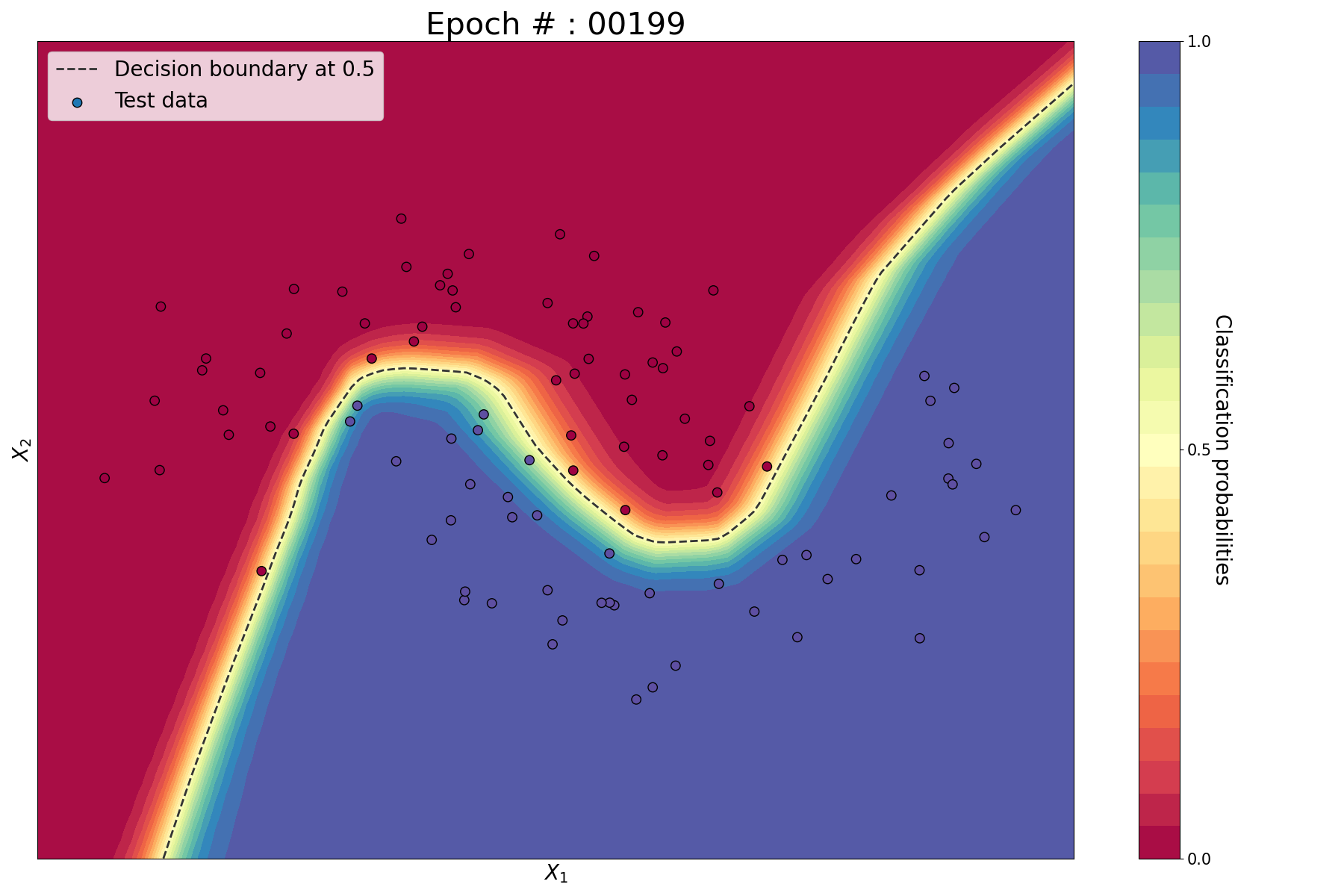
Here is a nice visualisation of what’s happening in an ANN during training. It lets you choose the input dataset, the type of problem (classification or regression), the training parameters (learning rate, activation function, regularization, etc…) and visualise the output.
Introduction
The simplest form of ANN is called Feedforward Neural Network (FNN), where a number of simple processing units (neurons) are organized in layers. Every neuron in a layer is connected with all the neurons in the previous layer. These connections are not all equal: each connection may have a different strength or weight. The weights on these connections encode the knowledge of a network. An FNN with one layer is called a Single-Layer Perceptron (SLP), an FNN with more than one layer is called… a Multi-Layer Perceptron. We will start very simple and explain how the Single-Layer Perceptron works for a classification problem.
A bit of theory
The architecture of the SLP is as follows,
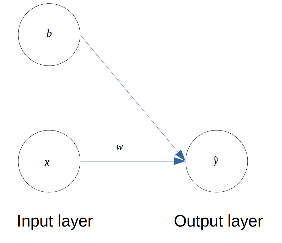 Architecture of a Single-Layer Perceptron
The SLP maps an input \(x\) (there is only one feature here) to a predicted output \(\hat{y}\). We define a weight \(w\) and a bias \(b\) between the 2 layers. The goal is to determine the weight and the bias that minimise a cost function that we will define later.
\(\hat{y}\) is the output of an activation function such as the Sigmoid function. This function squashes a real number into the [0, 1] interval. If the real number is negative, the output is close to 0 and if it is positive, the output is close to 1.
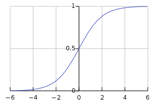 The Sigmoid function – Source
We can write the predicted output as follows,
\[\hat{y} = \sigma(z)\]From the network architecture, we get \(z = xw + b\).
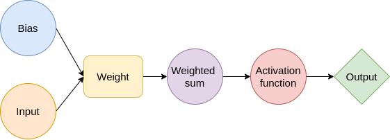
Since a diagram is worth a thousand words, here is a graphical explanation of the process.
In order to identify the optimal values for the weight and bias, we need to define a cost function \(J\). In this case, we will use the Mean Square Error (MSE), which is a common metric for classification problems but we could also use other ones.
\[J = \frac{1}{m}\sum_{i=1}^{m}(\hat{y}_i-y_i)^2\]where \(m\) is the number of observations, \(y\) is the label of each observation and \(\hat{y}\) is the output predicted by our network.
In order to minimise our cost function \(J\), we will apply the method of the Gradient Descent to the weight.
\[w := w - \alpha \frac{dJ}{dw}\]where \(\alpha\) is the learning rate.
We will use the chain rule of differentiation to calculate the gradient.
\[\frac{dJ}{dw} = \frac{dJ}{d\hat{y}} \frac{d\hat{y}}{dz} \frac{dz}{dw}\]Using previous equations, we can calculate each of the terms.
\[\begin{align*} \frac{dJ}{d\hat{y}} &= \frac{2}{m}(\hat{y}-y) \\ \frac{d\hat{y}}{dz} &= \sigma'(z) = \sigma(z) (1 - \sigma(z)) \\ \frac{dz}{dw} &= x \end{align*}\]We can do the same for the bias. The Gradient Descent is:
\[b := b - \alpha \frac{dJ}{db}\]The chain-rule gives:
\[\frac{dJ}{db} = \frac{dJ}{d\hat{y}} \frac{d\hat{y}}{dz} \frac{dz}{db}\]And finally we have:
\[\begin{align*} \frac{dJ}{d\hat{y}} &= \frac{2}{m}(\hat{y}-y) \\ \frac{d\hat{y}}{dz} &= \sigma'(z) = \sigma(z) (1 - \sigma(z)) \\ \frac{dz}{db} &= 1 \end{align*}\]If we put everything together, the weight and bias update becomes:
\[\begin{align*} w &:= w - \alpha \frac{2}{m}(\hat{y}-y) \sigma(z) (1 - \sigma(z)) x \\ b &:= b - \alpha \frac{2}{m}(\hat{y}-y) \sigma(z) (1 - \sigma(z)) \end{align*}\]That’s it! If we iterate the process enough times, the cost function will decrease and the weight and bias will converge to their optimal values.
In the next article, we will add a hidden layer between between the input and output layer to illustrate how the weights and biases are adjusted using Backpropagation.


Leave a comment